Best city for data scientists today according to two variables harvested with rvest
Some cities are more appealing for a data scientist to live than others. Several websites list best cities for data scientists, but their lists don’t agree and their methods are not explained, so the quality of the analysis and ability to determine which individuals their results can be inferred to are limited.
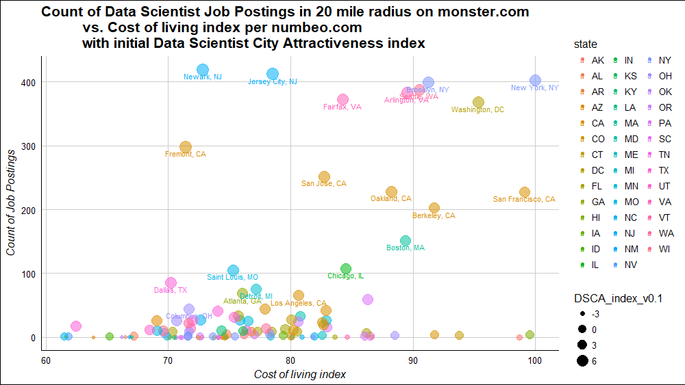
So here I set up to develop a reproducible, if not quite complete, measure of data scientist city attractiveness. Number of jobs for data scientists and cost of living may be two important variables. Using R’s rvest package, we can scrape from the web necessary information to get an idea how cities look in terms of these two. Got to DSCA index v0.1 shown above with top 21 cities labeled.
Bottom Line Up Front: Eight large hiring metros stand out, and less expensive cities within their communing distance look best by these variables. In particular, Newark, NJ, as cheap and close to lots of data scientist jobs, has the highest value in DSCA index v0.1. These two variables alone and the sources I chose show some interesting initial results, but they don’t seem to capture a complete picture, so more work is needed before getting a reliable reproducible index.
1. How many Data Scientist jobs are there in a given city?
One approach to see how many jobs a city has is search monster.com. “Data” and “scientist” can be keywords in other jobs, but I really want to know how many jobs with the words “Data Scientist” in the title are posted in each city. In this case for Portland, OR, I want a function that will return number 24.
This approach has limitations:
- Job postings do not represent people currently employed as a data scientist
- Some cities may fill and close these postings faster than others, so would appear to have fewer postings using one slice in time than say unique postings in a month
- Biases in favor of companies that post on Monster.com
- Over-counting from duplicates
- Under-counting for posts hiring for multiple positions
In any case, let’s use this as a proxy and see what shakes out. First step is to get a function that works to return 24 on just one city. In my browser, this search’s URL has an extra “&jobid=…” section to point at the first listed job and can be removed, so that for Portland, OR its minimal moster.com Data Scientist URL is:
url <- 'https://www.monster.com/jobs/search/?q=__22data-scientist__22&where=Portland__2C-OR'
We know we want this number 24. To get to it, http://selectorgadget.com/ offers a nice utility. You “install” it by adding a bookmark available there. Then when navigated to a page you want to scrape, click the bookmark to find a best tag to identify your website’s component you need. Clicking on 24 here, slectorgadget shows it’s in '.title' and so are 31 other elements.
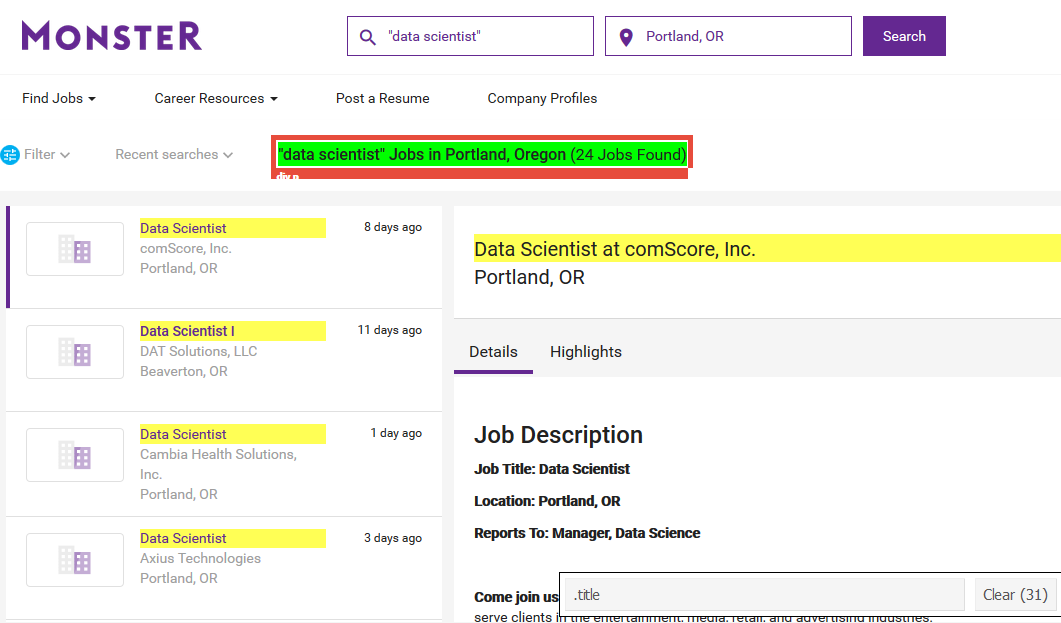
I only need the first one so click on one of the yellow ones to turn it red. Now selectorgadget has narrowed down to my best extractable tag, '.navigation-content .title'
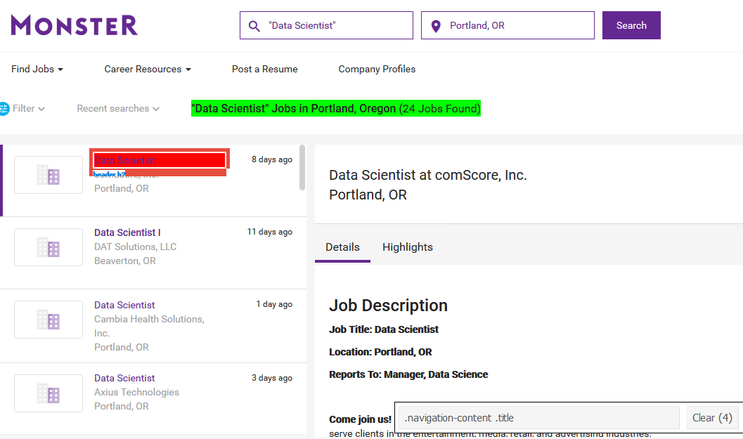
As a recap, what we’ve figured out is the html tags surrounding text we need to extract from this page. Using rvest library, we can use this information to harvest this page’s “most nutritious” content,
webpage <- read_html(url)
titles_html <- html_nodes(webpage, '.navigation-content .title')
titles_html

#{xml_nodeset (3)}
#[1] <h2 class="title">Filter your search</h2>
#[2] <p class="title">\r\n            <b>\r\n                 "data scientist" J ...
#[3] <h2 class="title">Get "data scientist" jobs in Portland as soon as they're  ...

# looks like it's the second element

library(tidyverse) # for dplyr, ggplot2, and purrr
titles_html[2] %>% html_text()
#[1] "\r\n            \r\n                 \"data scientist\" Jobs in Portland, Oregon \r\n            \r\n(24 Jobs Found)        "
Can see my goal number comes after a parenthesis “(“. So using ever-handy regex cheat sheet at http://www.rstudio.com/wp-content/uploads/2016/09/RegExCheatsheet.pdf we can extract only the number 24
library(stringr)

titles_html[2] %>%
  html_text() %>%
  str_extract('\\([0-9]*') %>%
  str_replace('\\(', '') %>%
  as.numeric()
#[1] 24
Cool, that worked. Let’s try a second city.
2. Expanding your scrape to additional cities
The obvious next city to try is Columbus, OH. Running a monster.com search on it shows the format of the url string https://www.monster.com/jobs/search/?q=__22Data-Scientist__22&where=Columbus__2C-OH simply replaces the city and state. Also, if we run the above code changing only its city and state we expect number 44 returned.
Indeed that is what happens. Here it has been piped for easier understanding
'https://www.monster.com/jobs/search/?q=__22data-scientist__22&where=Columbus__2C-OH' %>%
  read_html() %>%
  html_nodes('.navigation-content .title') %>%
  nth(2) %>%
  html_text() %>%
  str_extract('\\([0-9]*') %>%
  str_replace('\\(', '') %>%
  as.numeric()
#[1] 44
Next step, create a function that takes a city and state and returns a job count. Now two issues arise when trying to expand to other cities. We have multi name cities, such as Los Angeles, CA and Salt Lake City, UT. We need to know how monster represents those. We also have cities with no data scientist jobs available, such as Anchorage, AK. Let’s take a look.
Los Angeles’s url is https://www.monster.com/jobs/search/?q=__22Data-Scientist__22&where=Los-Angeles__2C-CA&jobid=195858182. Now we can remove the &jobid=... part and note the space is a dash. Similarly with Salt Lake City, https://www.monster.com/jobs/search/?q=__22Data-Scientist__22&where=Salt-Lake-City__2C-UT&jobid=814cce32-0bd4-41b3-91cc-6789f09ffdea it adds a dash in both spaces. These can be handled with stringr’s str_replace().
As for Data Science job postings in Alaska’s largest city, what you see in parenthesis isn’t a number, so it will return as NA.
We can handle that with an if(is.na()). And a function that works looks like this:
get_job_count <- function(city, state){
  city_dashed <- str_replace_all(city, '\\ ', '\\-')
  job_count <- paste0('https://www.monster.com/jobs/search/',
         '?q=__22data-scientist__22',
         '&where=',
         city_dashed,
         '__2C-',
         state) %>%
    read_html() %>%
    html_nodes('.navigation-content .title') %>%
    nth(2) %>%
    html_text() %>%
    str_extract('\\([0-9]*') %>%
    str_replace('\\(', '') %>%
    as.numeric()
  if(is.na(job_count)){
    job_count <- 0
  }
  data_frame(job_count)
}

get_job_count("Columbus", "OH")
# A tibble: 1 x 1
#  job_count
#      <dbl>
#1      44.0

get_job_count("Anchorage", "AK")
# A tibble: 1 x 1
#  job_count
#      <dbl>
#1         0

get_job_count("Salt Lake City", "UT")
# A tibble: 1 x 1
#  job_count
#      <dbl>
#1      12.0
It returns a tibble data frame with the expected number. Can see this is close to being iterable on every city we want to look up. We’re going to be doing a right join essentially on city cost of living data, so let’s get that now, and use that list to feed this function.
3. Scrape cost of living data
Cost of living per city indexed so that New York City is 1.00 is available at https://www.numbeo.com/cost-of-living/. This website appears to “croudsource” their cost of living data, so it’s going to be biased. Again we just need a rough idea, so let’s start with this.
Now monster only takes cities in the US, so let’s filter numbeo to Northern America at: https://www.numbeo.com/cost-of-living/region_rankings.jsp?title=2017®ion=021. We need two fields, the city, and the cost of living index. Here I pulled in columns individually. rvest does have an html_table() function, but it doesn’t work on some types of tables.
Using selectorgadget we can get the name of the city column.
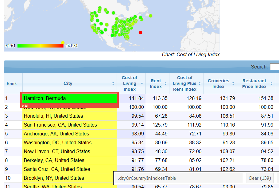
The cost of living index is a bit more complicated. Because this table is sorted by that column, clicking on it says it’s .sorting_1 but this won’t run in rvest. Instead one needs to sort by a different column to figure out the tag is td:nth-child(3).
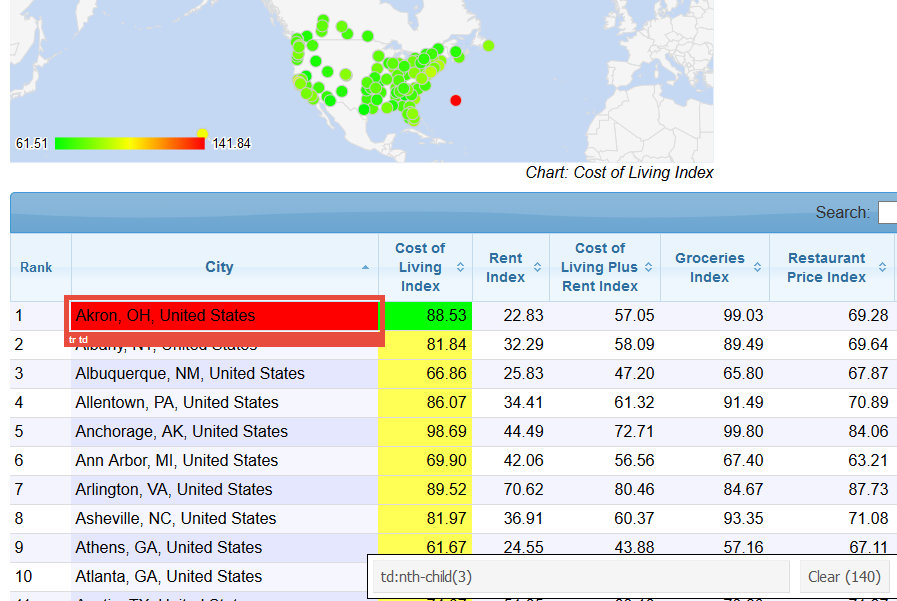
That brings in an extra row, so need to remove it.
cities <- 'https://www.numbeo.com/cost-of-living/region_rankings.jsp?title=2017®ion=021' %>%
read_html() %>%
html_nodes('.cityOrCountryInIndicesTable') %>%
html_text()
cost_of_living_index <- 'https://www.numbeo.com/cost-of-living/region_rankings.jsp?title=2017®ion=021' %>%
read_html() %>%
html_nodes('td:nth-child(3)') %>%
html_text()
# remove the top row
cost_of_living_index <- cost_of_living_index[-1]
# combine them
cities_to_check <- cbind(cities, cost_of_living_index) %>% as.data.frame
head(cities_to_check)
# cities cost_of_living_index
#1 Hamilton, Bermuda 141.84
#2 New York, NY, United States 100.00
#3 Honolulu, HI, United States 99.54
#4 San Francisco, CA, United States 99.14
#5 Anchorage, AK, United States 98.69
#6 Washington, DC, United States 95.34
Now again, unfortunately monster can’t find any jobs in Bermuda, and it also can’t take Canada, so let’s filter to US only and do some cleaning to prepare to run in the get_job_count function.
cities_to_check_cleaned
 <- cities_to_check %>%
  filter(str_detect(cities, "United States")) %>%
  separate(cities, c('city', 'state', 'country'), sep = ",") %>%
  # need sep or else it splits on spaces
  mutate(state = str_trim(state),
         cost_of_living_index =
           as.numeric(as.character(cost_of_living_index))) %>%
  select(city, state, cost_of_living_index)

head(cities_to_check_cleaned)
#           city state cost_of_living_index
#1      New York    NY               100.00
#2      Honolulu    HI                99.54
#3 San Francisco    CA                99.14
#4     Anchorage    AK                98.69
#5    Washington    DC                95.34
#6     New Haven    CT                93.75
4. Combine both sources
There are two inputs to the get_job_count() function, city and state, so a good choice is purrr’s map2 function. Let’s do a quick check on a subset of these cities first
cities_to_check_cleaned_short <- cities_to_check_cleaned[1:4, ]

map2_df(.x = cities_to_check_cleaned_short$city,
        .y = cities_to_check_cleaned_short$state,
        .f = get_job_count)
# A tibble: 4 x 1
#  job_count
#      <dbl>
#1    402
#2      4.00
#3    227
#4      0
It seems to work and return a data frame with numbers as expected, including a 0 for Anchorage, AK. Let’s run it on all listed cities and recombine into one data frame,
job_count <- map2_df(.x = cities_to_check_cleaned$city,
                     .y = cities_to_check_cleaned$state,
                     .f = get_job_count)

dim(job_count)
#[1] 112   1

dim(cities_to_check_cleaned)
#[1] 112   3

# same number of rows

count_by_city <- bind_cols(cities_to_check_cleaned, job_count) %>%
  mutate("City Name" = paste0(city, ", ", state),
         "City Name" = str_replace(`City Name`, '\\-', '\\ '))
head(count_by_city)
#           city state cost_of_living_index job_count         City Name
#1      New York    NY               100.00       402      New York, NY
#2      Honolulu    HI                99.54         4      Honolulu, HI
#3 San Francisco    CA                99.14       227 San Francisco, CA
#4     Anchorage    AK                98.69         0     Anchorage, AK
#5    Washington    DC                95.34       368    Washington, DC
#6     New Haven    CT                93.75         3     New Haven, CT
These are arranged by cost of living index. How about by job count?
count_by_city %>%
   arrange(desc(job_count)) %>%
   top_n(10, job_count)
#          city state cost_of_living_index job_count       City Name
#1       Newark    NJ                72.84       419      Newark, NJ
#2  Jersey City    NJ                78.53       412 Jersey City, NJ
#3     New York    NY               100.00       402    New York, NY
#4     Brooklyn    NY                91.25       399    Brooklyn, NY
#5      Seattle    WA                90.54       388     Seattle, WA
#6    Arlington    VA                89.52       383   Arlington, VA
#7      Fairfax    VA                84.26       372     Fairfax, VA
#8   Washington    DC                95.34       368  Washington, DC
#9      Fremont    CA                71.42       298     Fremont, CA
#10    San Jose    CA                82.75       252    San Jose, CA
5. Analysis of best city for data scientists
That’s how it looks. How can we combine cost of living and number of job postings to find one best city? A good place to start is a scatterplot. If filtering to cities with more than 20 postings,
library(ggthemes)
count_by_city %>%
  arrange(desc(job_count)) %>%
  filter(job_count >= 20) %>%
  ggplot(aes(x = cost_of_living_index, y = job_count,
             label = `City Name`, color = state)) +
  geom_point() +
  geom_text(vjust = 1, size = 3) +
  theme_gdocs() +
  ylab('Count of Job Postings') +
  xlab('Cost of living index') +
  ggtitle('Count of Data Scientist Job Postings in 20 mile radius on Monster.com
          vs. Cost of living index per numbeo.com
          for US Cities with 20+ Job Postings')
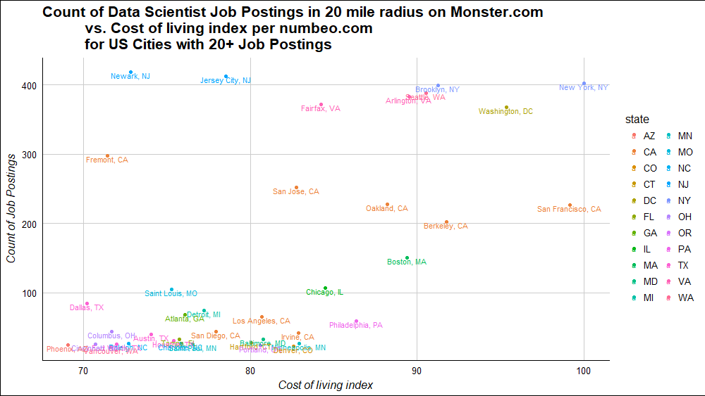
Colors by state are not the most useful but do show relation between these cities - for example all the Bay Area brown ones between 200 and 300.
Finally, to try to arrive at some intuitive ranking of cities, I’ve reduced these two variables into a one-dimensional Data Scientist City Attractiveness index.
`DSCA_index` = log(job_count + .1) / cost_of_living_index * 100
It may be simplistic, but a starting point, a null hypothesis, if you will, of what matters when choosing a city to live in as a data scientist. Final results…
count_by_city %>%
  mutate(`DSCA_index` = log(job_count + .1) / cost_of_living_index * 100) %>%
  arrange(desc(`DSCA_index`)) %>%
  top_n(20) %>%
  select(cost_of_living_index:DSCA_index) %>%
  mutate(`City Name` = reorder(`City Name`, DSCA_index)) %>%
  ggplot(aes(`City Name`, DSCA_index, fill = 1)) +
  geom_bar(stat = "identity", show.legend = FALSE) +
  coord_flip() +
  labs(x = "City",
       y = "DSCA index = exp(Job Posting Count) / Cost of Living Index",
       title = "Hypothesis Generation of top 20 cities to live as a Data Scientist")
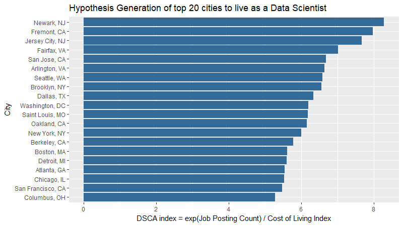
Newark, NJ takes first place!

The scatterplot at top of this post shows all 112 US cities with a cost of living index on numbeo. Cities above 5 on the index are labeled, cities lower are not.
6. Conclusion
NYC, Seattle, DC, Bay Area, Boston, Chicago, St. Louis, and Dallas have the most data scientist monster.com job postings, standing out as the eight largest hiring metros as of the time of this scrape. Some questions about data quality of both data sources remain, such as duplicate postings or San Jose being cheaper to live in than Oakland. So would take this index with a grain of salt.
Also, even if data reliability questions are addressed, these are obviously not the only two numbers that matter. A quality-of-data-scientist-life index might consider more relevant variables than jobs and cost of living alone. So obvious areas of improvement include:
- crime stats
- livability indices
- numbeo’s cost of living plus rent index
- average commute time to the jobs in the 20 mile radius
- smaller radii
- total population of metro area
- college educated population
- quantitative masters educated population
- natural beauty and low pollution
- small cities with many openings
- distribution of data scientist salaries
- sentiment of reviews of job experience as a data scientist
- monster.ca for Canadian postings
- interpretability of index
DSCA v0.1 code can be found at: https://github.com/dgarmat/data_scientist_city_attractiveness_index

