
ImageNet needs more Wild Boar Photos
Is your deep convolutional network misclassifying images? You can find out why with a heatmap of class activation overlaid on its misclassified pictures.
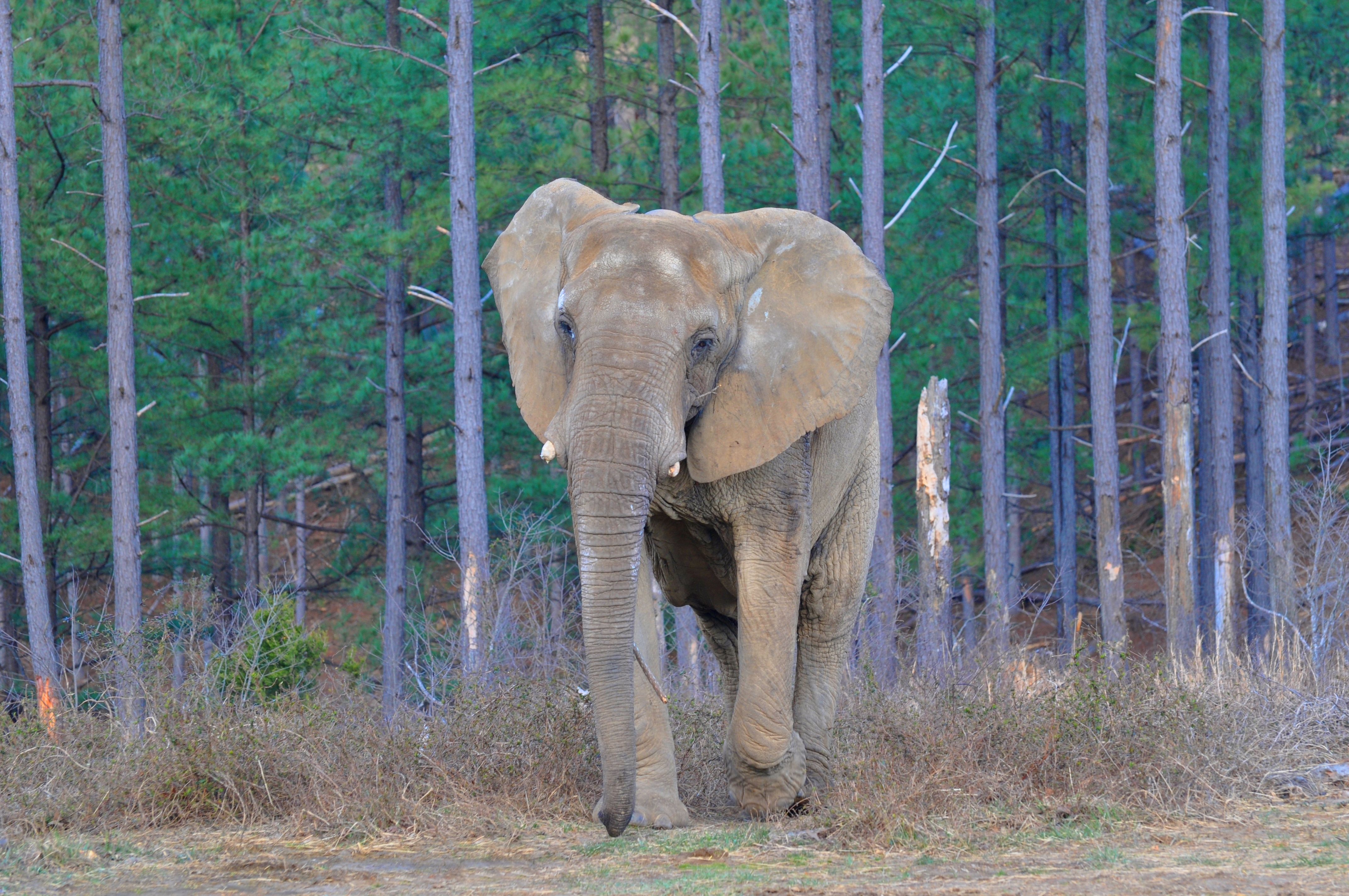
A heatmap overlay shows parts of an image most activated in a neural network’s last convolutional layer. In this African elephant picture, the top-most convolutional layer of the VGG16 architecture turns the photo into a 14x14 grid highlighting blocks with strongest African_elephant activation:

Original image source: elephants.com - African elephant Flora
What it’s saying with a yellow-green splotch is “Look! There’s an African elephant here!” The learner returns a score of 46%, quite high for a blink-of-an-eye judgment with 1000 objects to choose from and even locates that object in the picture correctly. Impressive.
imagenet_decode_predictions(preds, top = 3)[[1]]
#  class_name class_description      score
#1  n02504458  African_elephant 0.46432969
#2  n02437312     Arabian_camel 0.29539737
#3  n01871265            tusker 0.07210348
Shaded parts of this photo have at least some activation to class African_elephant. These show the elephant’s face and nearby foliage are what distinguish it from an Indian elephant and other classes, like a strawberry or an aircraft carrier. Parts of the photo that have 0 activation on the corresponding heatmap show up as non-shaded, which can be verified from a visualization of the activation heatmap:

or printing it out as a numeric matrix:
round(heatmap, 2)
#      [,1] [,2] [,3] [,4] [,5] [,6] [,7] [,8] [,9] [,10] [,11] [,12] [,13] [,14]
# [1,] 0.00 0.00 0.02 0.02 0.01 0.00 0.00 0.00 0.00  0.00  0.00  0.00  0.00  0.00
# [2,] 0.00 0.01 0.00 0.00 0.00 0.00 0.00 0.00 0.00  0.00  0.00  0.00  0.00  0.00
# [3,] 0.00 0.00 0.00 0.00 0.00 0.00 0.00 0.00 0.00  0.00  0.00  0.00  0.00  0.00
# [4,] 0.00 0.00 0.05 0.00 0.00 0.00 0.00 0.00 0.00  0.00  0.00  0.00  0.00  0.00
# [5,] 0.00 0.00 0.09 0.07 0.26 0.00 0.11 0.13 0.07  0.16  0.00  0.00  0.00  0.00
# [6,] 0.00 0.00 0.01 0.04 0.30 0.24 0.69 0.63 0.41  0.12  0.04  0.00  0.00  0.00
# [7,] 0.00 0.00 0.01 0.04 0.14 0.14 0.55 0.72 0.92  0.23  0.06  0.00  0.00  0.00
# [8,] 0.00 0.00 0.00 0.01 0.00 0.03 0.61 0.98 1.00  0.22  0.00  0.00  0.00  0.00
# [9,] 0.00 0.00 0.02 0.01 0.00 0.00 0.30 0.27 0.31  0.00  0.00  0.00  0.02  0.00
#[10,] 0.00 0.00 0.04 0.04 0.01 0.00 0.01 0.00 0.02  0.00  0.00  0.02  0.04  0.01
#[11,] 0.00 0.00 0.10 0.09 0.07 0.06 0.10 0.00 0.00  0.00  0.00  0.03  0.05  0.04
#[12,] 0.01 0.14 0.13 0.13 0.11 0.11 0.10 0.00 0.00  0.08  0.09  0.12  0.08  0.08
#[13,] 0.13 0.13 0.15 0.14 0.12 0.10 0.08 0.00 0.03  0.11  0.11  0.15  0.12  0.11
#[14,] 0.04 0.06 0.06 0.04 0.00 0.00 0.02 0.00 0.00  0.00  0.00  0.00  0.00  0.00
Detecting sources of errors
Here is another African elephant with huge ears above its neck, but this time the learner has misclassified it as a tusker with a score of 55% as opposed to 17% for African elephant. Tusker isn’t a terrible judgment. It’s a more generic group that includes wild boars but the classification is not as accurate as African elephant. What threw it off from making a more precise call? Let’s see.

Original image source: By Komar.de - Non-woven photomural Elephant
Looks like the top of the head and the back. Surprising it’s not the tusks. If we take a sample of ImageNet tusker training images, it quickly becomes obvious most tusker images are of elephants. In the first 25 tusker examples shown here, none look like wild boars.

So the cause of our misclassification is understandable, and a training set limitation error. A great first recourse would be to add to ImageNet other kinds of tuskers to better train that class.
imagenet_decode_predictions(preds, top = 3)[[1]]
#  class_name class_description     score
#1  n01871265            tusker 0.5496630
#2  n02504013   Indian_elephant 0.2749955
#3  n02504458  African_elephant 0.1732897
R Code
library(keras)
library(magick)
library(viridis)

model <- application_vgg16(weights = "imagenet") # keeping top
model # assumes input picture of size 224 x 224

img_path <- "images/African_elephant_1.jpg"

img <- image_load(img_path, target_size = c(224, 224)) %>%
  image_to_array() %>%
  array_reshape(dim = c(1, 224, 224, 3)) %>% # for batch of this size
  imagenet_preprocess_input() # channelwise color normalization

preds <- model %>% predict(img)
imagenet_decode_predictions(preds, top = 3)[[1]]

# get least likely classes for fun
tail(imagenet_decode_predictions(preds, top = 1000)[[1]])

max_class_nbr <- which.max(preds[1, ]) # is the class index

# if want to see second most class activations, get at which index
second_class_nbr <- which.max((preds[1, ])[-max_class_nbr]) # should be second
# add +1 if above the previous index number
second_class_nbr <- ifelse(second_class_nbr >= max_class_nbr,
                           second_class_nbr + 1,
                           second_class_nbr)


# visualize which parts of the image are most class 1 using Grad-CAM
elephant_output <- model$output[, max_class_nbr]
elephant_output <- model$output[, second_class_nbr]
last_conv_layer <- model %>% get_layer("block5_conv3")
grads <- k_gradients(elephant_output, last_conv_layer$output)[[1]]
pooled_grads <- k_mean(grads, axis = c(1, 2, 3))
iterate <- k_function(list(model$input),
                      list(pooled_grads, last_conv_layer$output[1,,,]))
c(pooled_grads_value, conv_layer_output_value) %<-% iterate(list(img))

for(i in 1:dim(conv_layer_output_value)[3]){
  conv_layer_output_value[,,i] <-
    conv_layer_output_value[,,i] * pooled_grads_value[[i]]
}

heatmap <- apply(conv_layer_output_value, c(1, 2), mean)

# normalize heatmap between 0 and 1
heatmap <- pmax(heatmap, 0)
heatmap <- heatmap / max(heatmap)

round(heatmap, 2)

write_heatmap <- function(heatmap, filename, width = 224, height = 224,
                          bg = "white", col = terrain.colors(12)){
  png(filename, width = width, height = height, bg = bg)
  op = par(mar = c(0, 0, 0, 0))
  on.exit({par(op); dev.off()}, add = TRUE)
  rotate <- function(x) t(apply(x, 2, rev))
  image(rotate(heatmap), axes = FALSE, asp = 1, col = col)
}

write_heatmap(heatmap, paste0(substr(img_path, 1, nchar(img_path) - 4), "_heatmap.png"))


image <- image_read(img_path)
info <- image_info(image)
geometry <- sprintf("%dx%d!", info$width, info$height)

pal <- col2rgb(viridis(20), alpha = TRUE)
alpha <- floor(seq(0, 255, length = ncol(pal)))
pal_col <- rgb(t(pal), alpha = alpha, maxColorValue = 255)
write_heatmap(heatmap, "elephant_overlay.png",
              width = dim(heatmap)[1], height = dim(heatmap)[2],
              bg = NA, col = pal_col)
image_read("elephant_overlay.png") %>%
  image_resize(geometry, filter = "quadratic") %>%
  image_composite(image, operator = "blend", compose_args = "20") %>%
  plot()

# then save output
image_read("elephant_overlay.png") %>%
  image_resize(geometry, filter = "quadratic") %>%
  image_composite(image, operator = "blend", compose_args = "20") %>%
  image_scale("x480") %>%
  image_convert(format = "jpg") %>%
  image_write(paste0(substr(img_path, 1, nchar(img_path) - 4), "_overlay.jpg"))


# reset the image to second elephant
img_path <- "images/African_elephant_2.jpg"
# then rerun the above from img <-