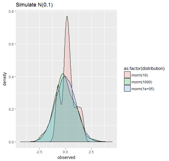
Hello World! Here's a Normal Distribution!

This code simulates Normal(0,1), and this visualization shows smaller samples can vary much more than large samples from the true distribution. Maybe it’s not a fascinating picture although there is a deep mystery or two in there. Can we know the truth? Isn’t everything we know based on a sample? Is everything we believe, like these three rnorm(), an incomplete story?

random simulations output

require(tidyverse)
require(tidyr)

random_simulations_1 <- tibble(rnorm(100000)) %>%
  gather %>% 
  rename(distribution = key, observed = value)

random_simulations_2 <- tibble(rnorm(1000)) %>%
  gather %>% 
  rename(distribution = key, observed = value) %>% 
  bind_rows(random_simulations_1)

random_simulations <- tibble(rnorm(10)#, rnorm(100)  
                             #runif(100)#,  
                             #rhyper(100, 100, 50, 10), 
                             #rbinom(100, 10, .5)
                             ) %>%
  gather %>% 
  rename(distribution = key, observed = value) %>% 
  bind_rows(random_simulations_2)

# note we've repeated three times, time for a function
# also note there are other distributions to try this on
# and really, it may ne nice to simulate a few pulls of 
#  the same size

ggplot(random_simulations, aes(observed, 
    fill = as.factor(distribution))) +
  geom_density(alpha = 0.2) + 
  labs(title = "Simulate N(0,1)")

Written on November 26, 2017